Molecular Orbital Theory

Objectives

By the end of this section, you will be able to:

• Outline the basic quantum-mechanical approach to deriving molecular orbitals from atomic orbitals
• Describe traits of bonding and antibonding molecular orbitals
• Calculate bond orders based on molecular electron configurations
• Write molecular electron configurations for first- and second-row diatomic molecules
• Relate these electron configurations to the molecules’ stabilities and magnetic properties

For almost every covalent molecule that exists, we can now draw the Lewis structure, predict the electron-pair geometry, predict the molecular geometry, and come close to predicting bond angles. However, one of the most important molecules we know, the oxygen molecule O₂, presents a problem with respect to its Lewis structure. We would write the following Lewis structure for O₂:

This electronic structure adheres to all the rules governing Lewis theory. There is an O=O double bond, and each oxygen atom has eight electrons around it. However, this picture is at odds with the magnetic behavior of oxygen. By itself, O₂ is not magnetic, but it is attracted to magnetic fields. Thus, when we pour liquid oxygen past a strong magnet, it collects between the poles of the magnet and defies gravity, as in [link]. Such attraction to a magnetic field is called paramagnetism, and it arises in molecules that have unpaired electrons. And yet, the Lewis structure of O₂ indicates that all electrons are paired. How do we account for this discrepancy?

Magnetic susceptibility measures the force experienced by a substance in a magnetic field. When we compare the weight of a sample to the weight measured in a magnetic field ([link]), paramagnetic samples that are attracted to the magnet will appear heavier because of the force exerted by the magnetic field. We can calculate the number of unpaired electrons based on the increase in weight.

Experiments show that each O₂ molecule has two unpaired electrons. The Lewis-structure model does not predict the presence of these two unpaired electrons. Unlike oxygen, the apparent weight of most molecules decreases slightly in the presence of an inhomogeneous magnetic field. Materials in which all of the electrons are paired are diamagnetic and weakly repel a magnetic field. Paramagnetic and diamagnetic materials do not act as permanent magnets. Only in the presence of an applied magnetic field do they demonstrate attraction or repulsion.

Water, like most molecules, contains all paired electrons. Living things contain a large percentage of water, so they demonstrate diamagnetic behavior. If you place a frog near a sufficiently large magnet, it will levitate. You can see videos of diamagnetic levitation in action.

Molecular orbital theory (MO theory) provides an explanation of chemical bonding that accounts for the paramagnetism of the oxygen molecule. It also explains the bonding in a number of other molecules, such as violations of the octet rule and more molecules with more complicated bonding (beyond the scope of this text) that are difficult to describe with Lewis structures. Additionally, it provides a model for describing the energies of electrons in a molecule and the probable location of these electrons. Unlike valence bond theory, which uses hybrid orbitals that are assigned to one specific atom, MO theory uses the combination of atomic orbitals to yield molecular orbitals that are delocalized over the entire molecule rather than being localized on its constituent atoms. MO theory also helps us understand why some substances are electrical conductors, others are semiconductors, and still others are insulators. The table below summarizes the main points of the two complementary bonding theories. Both theories provide different, useful ways of describing molecular structure.

Comparison of Bonding Theories

Valence Bond Theory	Molecular Orbital Theory
considers bonds as localized between one pair of atoms	considers electrons delocalized throughout the entire molecule
creates bonds from overlap of atomic orbitals (s, p, d…) and hybrid orbitals (sp, sp2, sp3…)	combines atomic orbitals to form molecular orbitals (σ, σ*, π, π*)
forms σ or π bonds	creates bonding and antibonding interactions based on which orbitals are filled
predicts molecular shape based on the number of regions of electron density	predicts the arrangement of electrons in molecules
needs multiple structures to describe resonance

Molecular orbital theory describes the distribution of electrons in molecules in much the same way that the distribution of electrons in atoms is described using atomic orbitals. Using quantum mechanics, the behavior of an electron in a molecule is still described by a wave function, Ψ, analogous to the behavior in an atom. Just like electrons around isolated atoms, electrons around atoms in molecules are limited to discrete (quantized) energies. The region of space in which a valence electron in a molecule is likely to be found is called a molecular orbital (Ψ²). Like an atomic orbital, a molecular orbital is full when it contains two electrons with opposite spin.

We will consider the molecular orbitals in molecules composed of two identical atoms (H₂ or Cl₂, for example). Such molecules are called homonuclear diatomic molecules. In these diatomic molecules, several types of molecular orbitals occur.

The mathematical process of combining atomic orbitals to generate molecular orbitals is called the linear combination of atomic orbitals (LCAO). The wave function describes the wavelike properties of an electron. Molecular orbitals are combinations of atomic orbital wave functions. Combining waves can lead to constructive interference, in which peaks line up with peaks, or destructive interference, in which peaks line up with troughs ([link]). In orbitals, the waves are three dimensional, and they combine with in-phase waves producing regions with a higher probability of electron density and out-of-phase waves producing nodes, or regions of no electron density.

There are two types of molecular orbitals that can form from the overlap of two atomic s orbitals on adjacent atoms. The two types are illustrated in the figure below. The in-phase combination produces a lower energy $σ_s$ molecular orbital (read as “sigma-s”) in which most of the electron density is directly between the nuclei. The out-of-phase addition (which can also be thought of as subtracting the wave functions) produces a higher energy $σ_s^*$ molecular orbital (read as “sigma-s-star”) molecular orbital in which there is a node between the nuclei. The asterisk signifies that the orbital is an antibonding orbital. Electrons in a σ_s orbital are attracted by both nuclei at the same time and are more stable (of lower energy) than they would be in the isolated atoms. Adding electrons to these orbitals creates a force that holds the two nuclei together, so we call these orbitals bonding orbitals. Electrons in the $σ_s^*$ orbitals are located well away from the region between the two nuclei. The attractive force between the nuclei and these electrons pulls the two nuclei apart. Hence, these orbitals are called antibonding orbitals. Electrons fill the lower-energy bonding orbital before the higher-energy antibonding orbital, just as they fill lower-energy atomic orbitals before they fill higher-energy atomic orbitals.

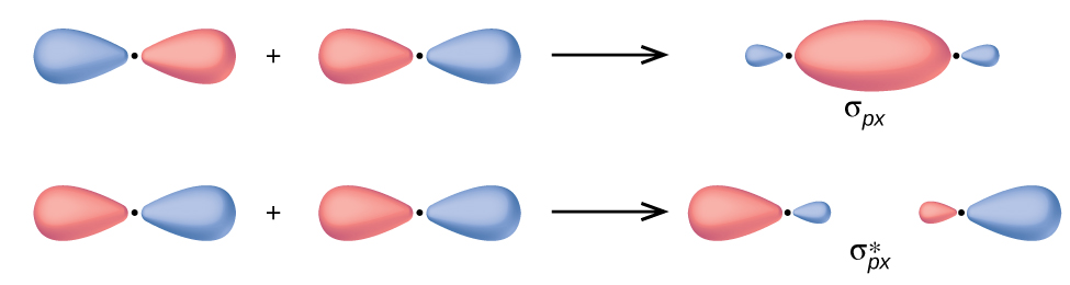
In p orbitals, the wave function gives rise to two lobes with opposite phases, analogous to how a two-dimensional wave has both parts above and below the average. We indicate the phases by shading the orbital lobes different colors. When orbital lobes of the same phase overlap, constructive wave interference increases the electron density. When regions of opposite phase overlap, the destructive wave interference decreases electron density and creates nodes. When p orbitals overlap end to end, they create σ and σ* orbitals (figure below). If two atoms are located along the x-axis in a Cartesian coordinate system, the two p_x orbitals overlap end to end and form $σ_{p_x}$ (bonding) and $σ_{p_x}^*$ (antibonding) (read as “sigma-p-x” and “sigma-p-x star,” respectively). Just as with s-orbital overlap, the asterisk indicates the orbital with a node between the nuclei, which is a higher-energy, antibonding orbital.

The side-by-side overlap of two p orbitals gives rise to a pi (π) bonding molecular orbital and a π* antibonding molecular orbital, as shown in the figure below. In valence bond theory, we describe π bonds as containing a nodal plane containing the internuclear axis and perpendicular to the lobes of the p orbitals, with electron density on either side of the node. In molecular orbital theory, we describe the π orbital by this same shape, and a π bond exists when this orbital contains electrons. Electrons in this orbital interact with both nuclei and help hold the two atoms together, making it a bonding orbital. For the out-of-phase combination, there are two nodal planes created, one along the internuclear axis and a perpendicular one between the nuclei.

In the molecular orbitals of diatomic molecules, each atom also has two sets of p orbitals oriented side by side (p_y and p_z), so these four atomic orbitals combine pairwise to create two π orbitals and two π* orbitals. The $π_{p_y}$ and $π_{p_y}^*$ orbitals are oriented at right angles to the $π_{p_z}$ and $π_{p_z}^*$ orbitals. Except for their orientation, the π_py and π_pz orbitals are identical and have the same energy; they are degenerate orbitals. The $π_{p_y}^*$ and $π_{p_z}^*$ antibonding orbitals are also degenerate and identical except for their orientation. A total of six molecular orbitals results from the combination of the six atomic p orbitals in two atoms: $σ_{p_x}$ and $σ_{p_x}^*$, $π_{p_y}$ and $π_{p_y}^*$, $π_{p_z}$ and $π_{p_z}^*$.

Further reading:

• Walter Kohn: Nobel Laureate
• Computational Chemistry in Drug Design