The goal of this section is to understand the electron orbitals (location of electrons in atoms), their different energies, and other properties. Quantum theory provides the best understanding of these concepts, which is crucial for understanding chemical bonding.
As described previously, electrons in atoms can exist only on discrete energy levels but not between them. The energy of an electron is quantized, meaning it can only have specific values. Electrons can jump from one energy level to another but not transition smoothly or stay between these levels.
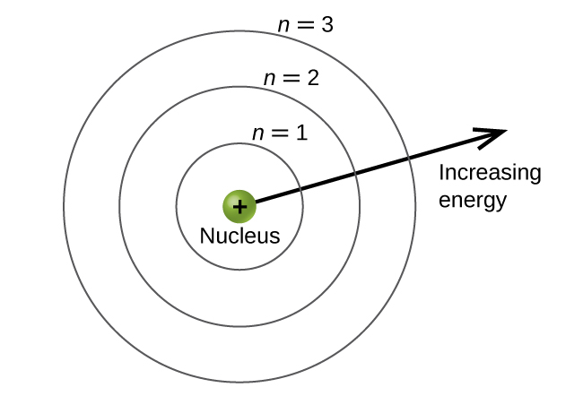
We label the energy levels with an n value, where n = 1, 2, 3, 4, and so on. Generally speaking, the energy of an electron in an atom is greater for greater values of n. We refer to this number, n, as the principal quantum number. The principal quantum number, n, defines the location of these energy level. It is essentially the same concept as the n in the Bohr atom description. Another name for the principal quantum number is the shell number. Think of the shells of an atom as concentric circles radiating out from the nucleus. Electrons in a specific shell tend to be found within its corresponding circular area.
The farther from the nucleus, the higher the shell number, and energy levels increase (Figure 1). Positively charged protons in the nucleus stabilize the electronic orbitals by electrostatic attraction. This attraction is essentially between the positive charges of the protons and the negative charges of the electrons. So the further away the electron is from the nucleus, the greater the energy it has.
Electronic Transitions
You can use this quantum mechanical model to examine electronic transitions. These occur when an electron moves from one energy level to another. When an electron transition to a higher energy level, it absorbs energy, and the energy change has a positive value. An atom absorbs a photon to gain the energy needed for a transition to a higher energy level. A transition to a lower energy level involves a release of energy, and the energy change is negative. This process is accompanied by emission of a photon by the atom. The following equation summarizes these relationships and is based on the hydrogen atom:
$$ΔE=E_{final}−E_{initial}$$
$$ΔE =−2.18×10^{−18}(\frac{1}{n_f^2}−\frac{1}{n_i^2})\;J$$
The values nf and ni are the final and initial energy states of the electron. The examples in the The Bohr Model page demonstrate calculations of such energy changes.
Principal and Secondary Quantum Numbers
The principal quantum number is one of three quantum numbers that characterize an orbital. An atomic orbital is a region in an atom, where an electron is most likely to be found. The quantum mechanical model specifies the probability of finding an electron in the three-dimensional space around the nucleus. We use Schrödinger equation here, as the model is based on its solutions. You’ll cover solving the Schrödinger equation in higher-levels courses.
Addiontionally, the principal quantum number defines the energy of an electron in a hydrogen or hydrogen-like atom or an ion (an atom or an ion with only one electron). It also indicates the general region in which discrete energy in multi-electron atoms and ions are located.
Another quantum number is l, the secondary (angular momentum) quantum number. It can be 0, 1, 2, …, n – 1, as long as it is an integer. Whereas the principal quantum number, n, defines the general size and energy of the orbital, the secondary quantum number l specifies the shape of the orbital. For example, an orbital with n = 1 can have only one value of l, l = 0, whereas n = 2 allows l = 0 and l = 1, and so on. Orbitals with the same value of l form a subshell.
Types of Orbitals
Orbitals with l = 0 are s orbitals, forming the s subshells. The value l = 1 corresponds to the p orbitals, and for given n, p orbitals constitute a p subshell (e.g., 3p if n = 3). The orbitals with l = 2 are d orbitals, followed by the f-, g-, and h-orbitals for l = 3, 4, and 5.
There are specific distances from the nucleus at which the probability density of finding an electron located in an orbital is zero. In other words, the value of the wavefunction ψ is zero at this distance for this orbital. A radius r with such a value is called a radial node. The number of radial nodes in an orbital is n – l – 1.
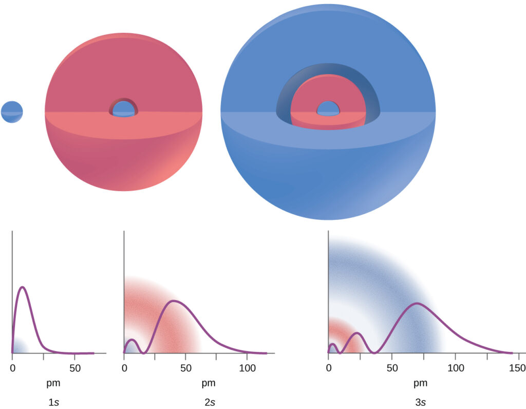
Consider the examples in Figure 2 above. The orbitals depicted are of the s type, thus l = 0 for all of them. The graphs of the probability densities shown are 1 – 0 – 1 = 0 places where the density is zero (nodes) for 1s (n = 1), 2 – 0 – 1 = 1 node for 2s, and 3 – 0 – 1 = 2 nodes for the 3s orbitals.
The s subshell electron density distribution is spherical and the p subshell has a dumbbell shape. The d and f orbitals are more complex. These shapes represent the three-dimensional regions where the elctron is most likely to be found.
Magnetic Quantum Number
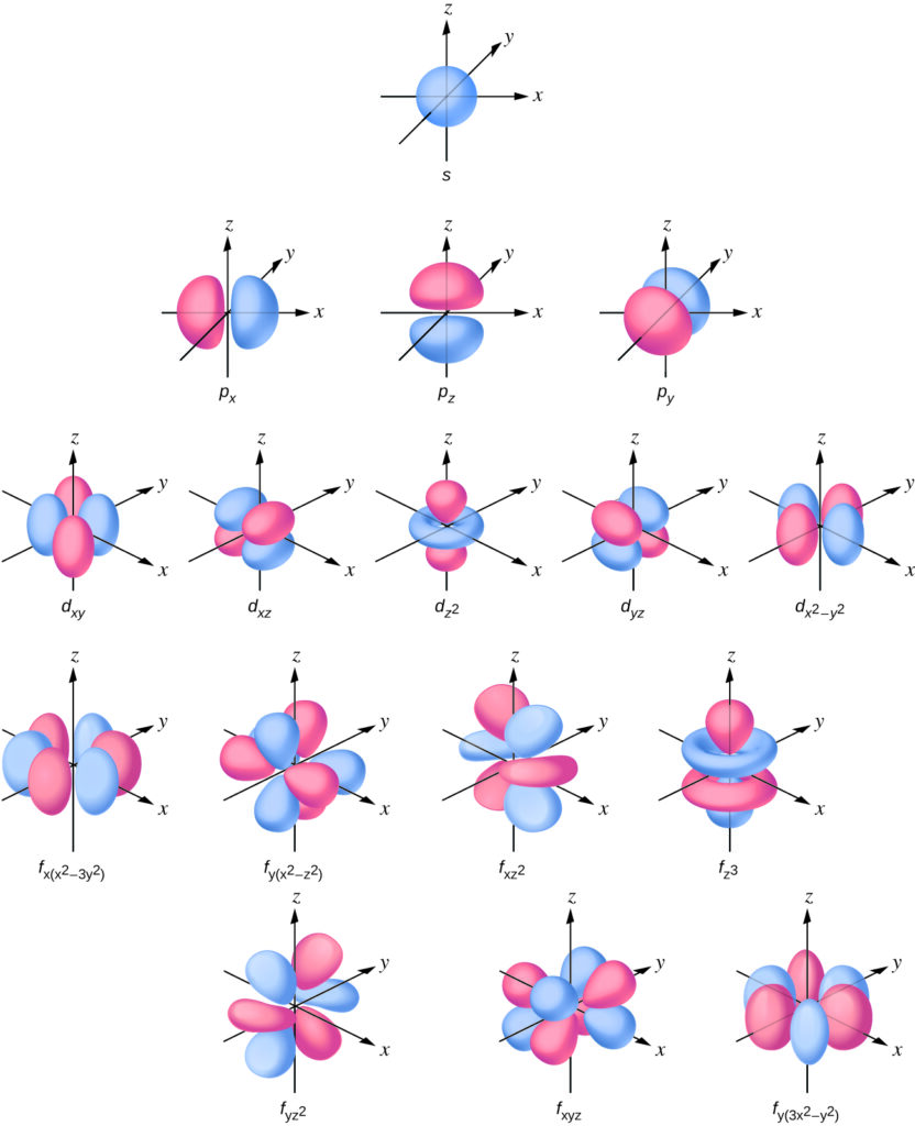
The magnetic quantum number, ml, describes the relative spatial orientation of a particular orbital. Generally speaking, ml can be equal to –l, –(l – 1), …, 0, …, (l – 1), l. The total number of possible orbitals with the same value of l (that is, in the same subshell) is 2l + 1. Thus, there is one s-orbital in an s subshell (l = 0), there are three p-orbitals in a p subshell (l = 1), five d-orbitals in a d subshell (l = 2), seven f-orbitals in an f subshell (l = 3), and so forth. The principal quantum number defines the general value of the electronic energy. The angular momentum quantum number determines the shape of the orbital. The magnetic quantum number specifies orbital’s orientation in space, as shown in Figure 3.
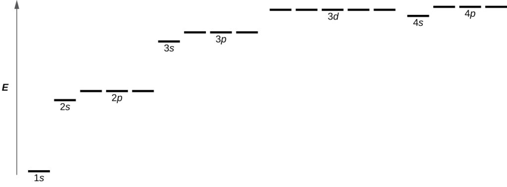
Figure 4 illustrates the energy levels for various orbitals. The number before the orbital name (such as 2s, 3p, and so forth) stands for the principal quantum number, n. The letter in the orbital name defines the subshell with a specific angular momentum quantum number l = 0 for s orbitals, 1 for p orbitals, 2 for d orbitals. Finally, there are more than one possible orbitals for l ≥ 1, each corresponding to a specific value of ml. We will explain why an energy level like 4s is lower than a 3d orbital in other topics.
Quantized Energy Levels and Principle Quantum Number
In the case of a hydrogen atom or a one-electron ion (such as He+, Li2+, and so on), energies of all the orbitals with the same n are the same. This phenomenon is known as degeneracy, and the energy levels for the same principal quantum number, n, are called degenerate orbitals. Yet , in atoms with more than one electron, electron–electron interactions eliminate degeneracy, causing orbitals that belong to different subshells have different energies, as shown on Figure 4. Orbitals within the same subshell are still degenerate and have the same energy.
While the three quantum numbers discussed in the previous paragraphs work well for describing electron orbitals, some experiments showed that they were not sufficient to explain all observed results. In the 1920s, scientist demonstrated that high-resolution examination of hydrogen-line spectra reveals some lines as pairs of closely spaced lines, not single peaks. This is the so-called fine structure of the spectrum, and it implies that there are additional small differences in energies of electrons even when they are located in the same orbital. These observations led Samuel Goudsmit and George Uhlenbeck to propose that electrons have a fourth quantum number. They called this the spin quantum number, or ms.
Electron Spin, Spin States and Quantum Mechanics
The other three quantum numbers, n, l, and ml, are properties of specific atomic orbitals that also define in what part of the space an electron is most likely to be located. Orbitals are a result of solving the Schrödinger equation for electrons in atoms. The electron spin is a different kind of property. It is a completely quantum phenomenon with no analogues in the classical realm. Addintionally solving the Schrödinger equation cannot derive it, and is does not related to the normal spatial coordinates (such as the Cartesian x, y, and z). Electron spin describes an intrinsic “rotation” or “spinning” of the electron. Each electron behaves like tiny magnet. You can also visualize an electron is as a tiny rotating object with angular momentum, or a loop with an electric current. However, this rotation or current does not appear in spatial coordinates.
The magnitude of the overall electron spin can only have one value. An electron can only “spin” in one of two quantized states. One is termed the α state, with the $z$ component of the spin being in the positive direction of the $z$ axis. This corresponds to the spin quantum number $m_s=\frac{1}{2}$. The other state is the β state, with the z component of the spin being negative and $m_s=-\frac{1}{2}$. Any electron, regardless of atomic orbital location, can only have one of two possible values of the spin quantum number. An external magnetic field causes electrons with $m_s=-\frac{1}{2}$ and $m_s=\frac{1}{2}$ to have different energies.
Magnetic Moment Behaviour, Energy Differences and Spectral Lines
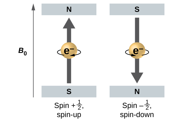
Figure 5 illustrates this phenomenon. An electron acts like a tiny magnet. For the spin quantum number $\frac{1}{2}$, the moment points up (in the positive direction of the z axis), while for $-\frac{1}{2}$, it spins down (in the negative z direction). A magnet has a lower energy when its magnetic moment aligns with the external magnetic field (the left electron in Figure 5). It has higher energy when the magnetic moment opposes the applied field.
An electron with $m_s=\frac{1}{2}$ has a slightly lower energy in an external field in the positive z direction, and an electron with $m_s=-\frac{1}{2}$ has a slightly higher energy in the same field. This is true even for an electron occupying the same orbital in an atom. A spectral line corresponds to a transition for electrons from the same orbital but with different spin quantum numbers. This results in two possible values of energy; thus, the line in the spectrum will show a fine structure splitting.