The previous discussion showed that the KMT qualitatively explains the behaviors described by the various gas laws. The postulates of this theory may be applied in a more quantitative fashion to derive these individual laws. To do this, we must first look at velocities and kinetic energies of gas molecules, and the temperature of a gas sample.
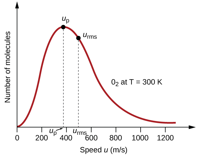
In a gas sample, individual molecules have widely varying speeds; however, because of the vast number of molecules and collisions involved, the molecular speed distribution and average speed are constant. This molecular speed distribution is known as a Maxwell-Boltzmann distribution, and it depicts the relative numbers of molecules in a bulk sample of gas that possesses a given speed ([link]).
The kinetic energy (KE) of a particle of mass (m) and speed (u) is given by: $$KE=\frac{1}{2}mu^2$$
Expressing mass in kilograms and speed in meters per second will yield energy values in units of joules (J = kg m2 s–2). To deal with a large number of gas molecules, we use averages for both speed and kinetic energy. In the KMT, the root mean square speed of a particle, urms, is defined as the square root of the average of the squares of the velocities with n = the number of particles:
$$u_{rms}=\sqrt{\overline{u^2}}=\sqrt{\frac{u_1^2+u_2^2+u_3^2+u_4^2+…}{n}}$$
The average kinetic energy for a mole of particles, KEavg, is then equal to:
$$KE_{avg}=\frac{1}{2}Mu_{rms}^2$$
where M is the molar mass expressed in units of kg/mol. The KEavg of a mole of gas molecules is also directly proportional to the temperature of the gas and may be described by the equation:
$$KE_{avg}=\frac{3}{2}RT$$
where R is the gas constant and T is the kelvin temperature. When used in this equation, the appropriate form of the gas constant is 8.314 J/mol⋅K (8.314 kg m2s–2mol–1K–1). These two separate equations for KEavg may be combined and rearranged to yield a relation between molecular speed and temperature:
$$\frac{1}{2}Mu_{rms}^2=\frac{3}{2}RT$$
$$u_{rms}=\sqrt{\frac{3RT}{M}}$$
Calculation of urms
Calculate the root-mean-square velocity for a nitrogen molecule at 30 °C.
Solution
Convert the temperature into Kelvin:
$$30°C+273=303\;K$$
Determine the molar mass of nitrogen in kilograms:
$$\frac{28.0\;\require{enclose}\enclose{horizontalstrike}{g}}{1\;mol}\times\frac{1\;kg}{1000\;\enclose{horizontalstrike}{g}}=0.028\;kg/mol$$
Replace the variables and constants in the root-mean-square velocity equation, replacing Joules with the equivalent kg m2s–2: $$u_{rms}=\sqrt{\frac{3RT}{M}}$$
$$u_{rms}=\sqrt{\frac{3(8.314\;J/mol\;K)(303\;K)}{(0.028\;kg/mol)}}=\sqrt{2.70×10^5\;m^2s^{−2}}=519\;m/s$$
Check Your Learning
Calculate the root-mean-square velocity for a mole of oxygen molecules at –23 °C.
Answer:
441 m/s
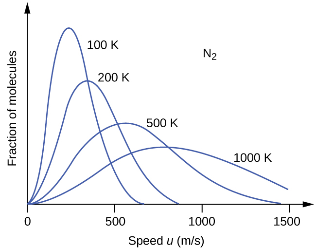
If the temperature of a gas increases, its KEavg increases, more molecules have higher speeds and fewer molecules have lower speeds, and the distribution shifts toward higher speeds overall, that is, to the right. If temperature decreases, KEavg decreases, more molecules have lower speeds and fewer molecules have higher speeds, and the distribution shifts toward lower speeds overall, that is, to the left. This behavior is illustrated for nitrogen gas in [link].
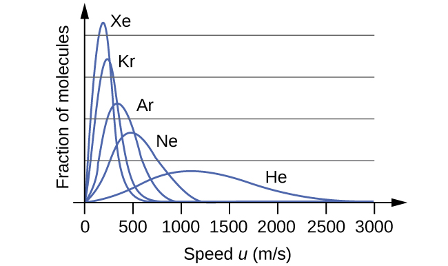
At a given temperature, all gases have the same KEavg for their molecules. Gases composed of lighter molecules have more high-speed particles and a higher urms, with a speed distribution that peaks at relatively higher velocities. Gases consisting of heavier molecules have more low-speed particles, a lower urms, and a speed distribution that peaks at relatively lower velocities. This trend is demonstrated by the data for a series of noble gases shown in [link].
The gas simulator may be used to examine the effect of temperature on molecular velocities. Examine the simulator’s “energy histograms” (molecular speed distributions) and “species information” (which gives average speed values) for molecules of different masses at various temperatures.