In order to reduce the uncertainty in their measurements, scientists will usually make repeated observations of any measurement (called replicate measurements, or replicates). Experimental error cannot always be eliminated, but it can be characterized and reduced by averaging over several measurements. The type of uncertainty in a measurement can be described by examining the accuracy and precision of the value.
Accuracy of Measured Values
The accuracy of a measurement reflects how close the measurement is to the “true” value. In some cases (like when you are measuring a sample with an unknown concentration), this “true” value is not known, so you will gauge your accuracy from other measurements (for example, a titration).
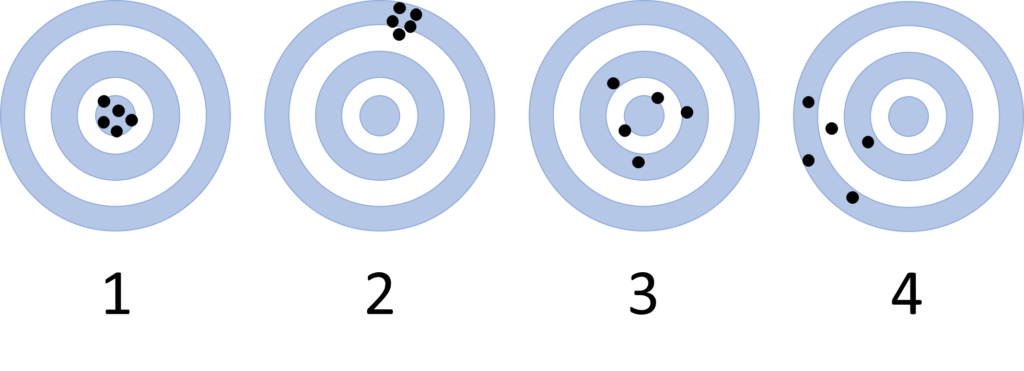
One way to visualize this is to imagine the measurements as hits on a dartboard, where the “true” value is the bullseye:

Target 3 also shows a more accurate result: though the hits are more spread out, they are still centered on the bullseye. Target 4 is again less accurate: the grouping of hits is far from the bullseye value.
Notice that the description of accuracy in these targets does not depend on how tightly grouped the hits are, just on how close they (or their collective average) are to the bullseye.
Expressing Accuracy
When the “true” value of a measurement is known, you can express the accuracy of a measurement with its percent error:
$$ \% \; error = \frac{\left| observed\; value-true\; value \right| }{true\; value} \times 100 \% $$
Percent error can be positive (the measured value is higher than the “true” value) or negative (the measured value is lower than the “true” value). Generally, a larger % error – either positive or negative – implies a less accurate measurement.
How much error is acceptable in your reported value depends on the nature of the measurement. In many first-year lab experiments, an accuracy of ~5% may be expected based on the experimental design and equipment used. A comparable measurement from a second-year analytical lab may have an expected accuracy of less than 0.5%.
Precision of Measured Values
The precision of a measurement describes the reproducibility of the value: if you took this measurement again, how similar will the two measurements be? One way to think about precision is as the spread or deviation of the measurements around their central (average) value. If we revisit the “bullseye” example from above:

The hits on Targets 1 and 2 are relatively precise: their “hits” are close together, and the dart thrower is hitting nearly the same spot each time. Targets 3 and 4 show less precise results: there is more scatter to the hits and they cover a wider range of values on the target.
Although we use the word precise in common English in several ways, in chemistry, precision or precise data refers specifically to this spread and repeatability of the measurements, as accuracy is described separately.
It is possible for data to be both accurate AND precise (as in Target 1 above), precise but not accurate (as in Target 2 above), accurate but not precise (as in Target 3 above), or neither accurate NOR precise (as in Target 4 above).
Expressing Precision
There are several ways to express the precision of a measurement numerically: through use of significant figures, by calculating the standard deviation of a set of data, or by using an error limit (or “error range”) to show the variability in the data.
As with accuracy, what is an acceptable value for the precision of your data depends on the type of measurement being made. For example, a typical pH meter will only give 2 or 3 significant figures in a result (i.e. $ pH =2.02 \pm 0.01 $), while correct use of a volumetric flask can give 4 or 5 significant figures in the final answer.(e.g. $ 100.0 \pm 0.1 \; mL $)
Significant Figures
All numerical values come with an implied precision based on how many digits we write into them. For example, you may measure a beaker to weigh 124.758 g, or buy a 2.0 m USB charging cable.
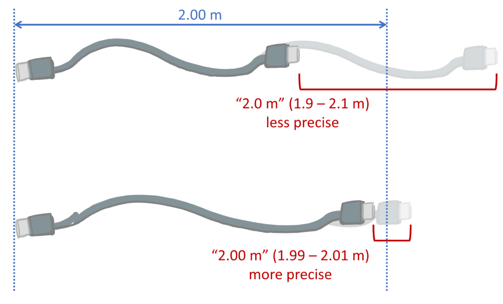
Following the conventions of reporting significant figures in our numbers, we would assume that these measurements as reported are repeatable to within $ \pm 1$ in the last reported digit. So, if I re-weighed the beaker I should expect a value between 124.757 – 124.759 g, or to measure the USB cable and find a value between 1.9 – 2.1 m.
A value that can be (correctly) expressed with more significant figures is more precise. Having more significant figures in the value means that the variation in the number is small compared to its overall value (e.g. the 2.0 m USB cable could be anywhere from 190 cm – 210 cm long. A 2.00 m cable would imply the cable should be within 199-201 cm – a more precise value, since there is less ‘spread’ over the potential measurements).

See more about significant figures.
Standard Deviation
The spread or scatter of experimental data around its average value can be described with the standard deviation (also called statistical precision), s. Standard deviation can be calculated for any data set with 3 or more data points:
$$ s=\sqrt{\frac{\sum_{i}{(M_{i} – \bar{M})^2}}{n-1}} $$
Where:
- Mi is an individual measurement or observed value
- $ \bar{M} $ is the mean (arithmetic average of all observed values)
- n is the total number of measurements
- $\sum_{i}{ } $ means “sum of” – in this case indicating to sum all of the available values of $ (M_{i} – \bar{M})^2 $.
A larger standard deviation indicates a lower precision in that measurement set (a larger ‘spread’ in the measurements). For more detail on using standard deviation as a measure of experimental uncertainty, see Chapter 4 in Analytical Chemistry 2.1 by D. Harvey.