Entropy and Microstates

Following the work of Carnot and Clausius, Ludwig Boltzmann developed a molecular-scale statistical model that related the entropy of a system to the number of microstates (W) possible for the system. A microstate is a specific configuration of all the locations and energies of the atoms or molecules that make up a system. The relation between a system’s entropy and the number of possible microstates is

$$S=klnW$$

where k is the Boltzmann constant, 1.38 $\times$ 10⁻²³ J/K.

As for other state functions, the change in entropy for a process is the difference between its final (S_f) and initial (S_i) values:

$$ΔS=S_f-S_i=klnW_f-klnW_i=kln\frac{W_f}{W_i}$$

For processes involving an increase in the number of microstates, W_f > W_i, the entropy of the system increases and ΔS > 0. Conversely, processes that reduce the number of microstates, W_f < W_i, yield a decrease in system entropy, ΔS < 0. This molecular-scale interpretation of entropy provides a link to the probability that a process will occur as illustrated in the next paragraphs.

Consider the general case of a system comprised of N particles distributed among n boxes. The number of microstates possible for such a system is n^N. For example, distributing four particles among two boxes will result in 2⁴ = 16 different microstates as illustrated in [Figure 2]. Microstates with equivalent particle arrangements (not considering individual particle identities) are grouped together and are called distributions. The probability that a system will exist with its components in a given distribution is proportional to the number of microstates within the distribution. Since entropy increases logarithmically with the number of microstates, the most probable distribution is therefore the one of greatest entropy.

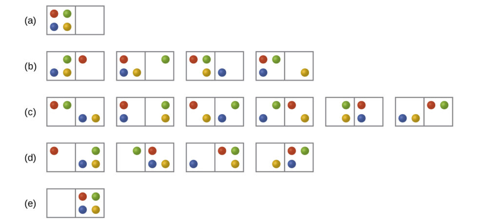
For this system, the most probable configuration is one of the six microstates associated with distribution (c) where the particles are evenly distributed between the boxes, that is, a configuration of two particles in each box. The probability of finding the system in this configuration is $\frac{6}{16}$ or $\frac{3}{8}$$.$ The least probable configuration of the system is one in which all four particles are in one box, corresponding to distributions (a) and (e), each with a probability of $\frac{1}{16}$$.$ The probability of finding all particles in only one box (either the left box or right box) is then ($\frac{1}{16}+\frac{1}{16})=\frac{2}{16}$ or $\frac{1}{8}$$.$

As you add more particles to the system, the number of possible microstates increases exponentially (2^N). A macroscopic (laboratory-sized) system would typically consist of moles of particles (N ~ 10²³), and the corresponding number of microstates would be staggeringly huge. Regardless of the number of particles in the system, however, the distributions in which roughly equal numbers of particles are found in each box are always the most probable configurations.

This matter dispersal model of entropy is often described qualitatively in terms of the disorder of the system. By this description, microstates in which all the particles are in a single box are the most ordered, thus possessing the least entropy. Microstates in which the particles are more evenly distributed among the boxes are more disordered, possessing greater entropy.

The previous description of an ideal gas expanding into a vacuum ([link]) is a macroscopic example of this particle-in-a-box model. For this system, the most probable distribution is confirmed to be the one in which the matter is most uniformly dispersed or distributed between the two flasks. Initially, the gas molecules are confined to just one of the two flasks. Opening the valve between the flasks increases the volume available to the gas molecules and, correspondingly, the number of microstates possible for the system. Since W_f > W_i, the expansion process involves an increase in entropy (ΔS > 0) and is spontaneous.

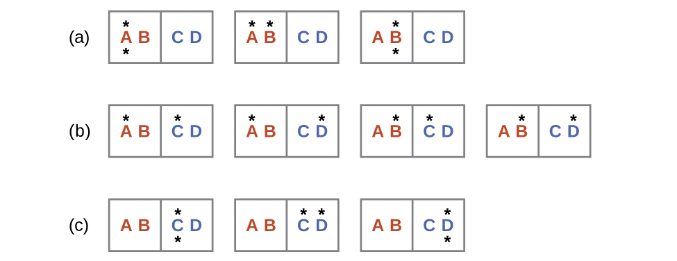
A similar approach may be used to describe the spontaneous flow of heat. Consider a system consisting of two objects, each containing two particles, and two units of thermal energy (represented as “*”) in [Figure 2]. The hot object is comprised of particles A and B and initially contains both energy units. The cold object is comprised of particles C and D, which initially has no energy units. Distribution (a) shows the three microstates possible for the initial state of the system, with both units of energy contained within the hot object. If one of the two energy units is transferred, the result is distribution (b) consisting of four microstates. If both energy units are transferred, the result is distribution (c) consisting of three microstates. Thus, we may describe this system by a total of ten microstates. The probability that the heat does not flow when the two objects are brought into contact, that is, that the system remains in distribution (a), is $\frac{3}{10}$$.$ More likely is the flow of heat to yield one of the other two distribution, the combined probability being $\frac{7}{10}$$.$ The most likely result is the flow of heat to yield the uniform dispersal of energy represented by distribution (b), the probability of this configuration being $\frac{4}{10}$. This supports the common observation that placing hot and cold objects in contact results in spontaneous heat flow that ultimately equalizes the objects’ temperatures. And, again, this spontaneous process is also characterized by an increase in system entropy.